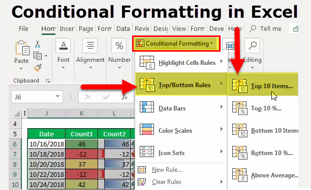
While learning about visualizing data in Excel spreadsheets, we have already learned about Working with Charts in Excel Workbook. Now, let us explore another feature of Conditional Formatting in Excel files. It is a useful and effective way of presenting information.
In this article, we will be learning the following features:
- Add Conditional Formatting in Excel Spreadsheet
- Delete Conditional Formatting in Excel Spreadsheet
- Update Conditional Formatting in Excel Spreadsheet
Add Conditional Formatting in Excel Spreadsheet
You can specify different parameters of the condition including the Type, Operator, Style, Cell Area, etc, and then call the API. The following C# .NET code snippet explains the steps to accomplish this requirement:
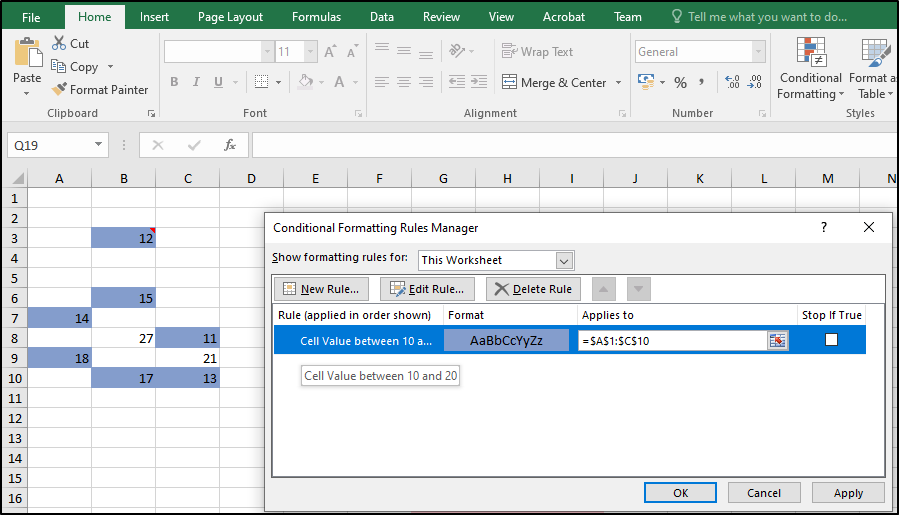
This code snippet will add conditional formatting to the specified cell area. You can notice the changed background color of cells that contain the value under a specific range.
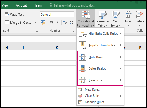
Moreover, Microsoft Excel offers three presets i.e. Data Bars, Color Scales, and Icon Sets. The following screenshot shows these presets. Fortunately, Aspose.Cells Cloud API supports all of these presets. Such features elevate the API to be the best fit for processing Excel spreadsheet files.
Delete Conditional Formatting in Excel Spreadsheet
You can delete any conditional formatting from an Excel workbook. Simply set the index of formatting and call the API. However, the index is zero-based so zero should be passed to delete first formatting and so on. Please use the following C# code snippet to delete the first occurrence of conditional formatting from the specified worksheet of the specific workbook:
Furthermore, you can also delete all conditional formatting from a worksheet in a single API call. Simply omit or comment out the index variable and the API will delete all the formatting from the specified worksheet.
Update Conditional Formatting in Excel Spreadsheet
You can update existing conditional formatting in an Excel file. For instance, let us update the Condition Area in the formatting we had added in the very first example of this article. You can notice in that screenshot as well that the area is set as A1:C10. Let us continue that example and further include E6:G8 cells. The following code snippet can be used to update the condition area:
The below screenshot highlights how the same condition is extended to another area specified in the code snippet.
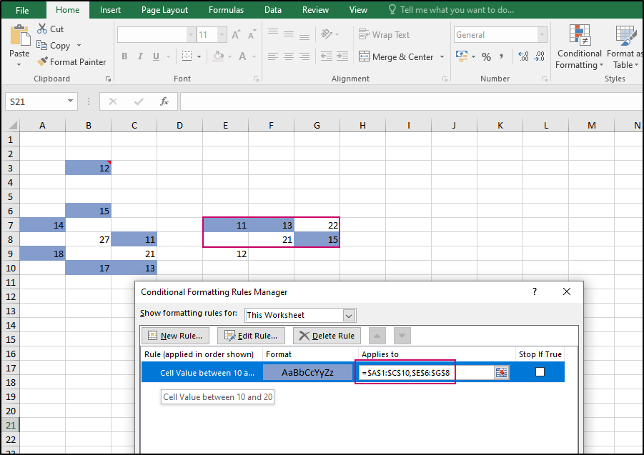
The highlighted area on this screenshot is an example of how the updating of the Condition Area works. The cells in range E6:G8 are now appended to the condition area.
Conclusion
In the above blog post, we have explored a few of the possibilities that you can utilize in your applications. You can further refer to API references, API documentation, and different SDKs of Aspose.Cells for Cloud API. We look forward to your feedback or suggestions at Free Support Forums. Cheers!